Physics-Based Simulation (BBP)

What BBP Adds

For qualifying earthquakes, Intensity Lab can replace an empirical synthetic ground motion (a signal statistically fitted to a single peak-acceleration number — see Physics Animation (Blender)) with a physics-based simulated seismogram computed by the SCEC Broadband Platform (BBP) version 22.4.0. The distinction matters: the empirical synthetic is fitted to a peak-acceleration number, whereas a BBP seismogram is computed from a rupture model propagating through a regional crustal velocity model.

BBP runs as a separately hosted, metered REST API (the bbpapi service). Intensity Lab's worker submits a scenario job and polls for the result; a job's heavy Fortran computation runs on an on-demand cloud instance, not on the Intensity Lab web server itself.

Building the Rupture (src) From ShakeMap Event Parameters

The pipeline builds a BBP scenario job (a "src" rupture description) directly from the USGS event parameters used everywhere else on this site:

• Fault geometry from the USGS moment tensor's first nodal plane (strike, dip, rake); when no moment tensor is published, a regional strike-slip default is used
• Fault dimensions from Wells & Coppersmith (1994) magnitude scaling, with the hypocenter centered down-dip at the USGS depth
• Method: Graves & Pitarka (GP), a hybrid broadband approach combining deterministic low-frequency wave propagation with a stochastic high-frequency component
• Rupture seed derived deterministically (via SHA-256, not Python's per-process-salted hash()) from the USGS event id, so re-running an event reproduces the same waveform across worker restarts

Selecting the 1D Velocity Model

A BBP velocity model is a layered one-dimensional crustal profile of seismic velocity and density, not a map — it can technically be applied anywhere, but it only physically describes the region it was built for. Intensity Lab installs several California regional velocity-model packages and routes each earthquake to the model whose native extent contains its epicenter:

• LABasin500 (“SoCal” on the map) — Los Angeles basin / Southern California
• Mojave500 (“Mojave”) — the Ridgecrest & Mojave / eastern Southern California corridor
• CentralCal500 (“CenCoast”) — Coast Ranges, Central Valley, Parkfield
• NoCal500 (“NoCal”) — San Francisco Bay Area and northward
• SouthernSierra500-2 (“Southern Sierra Nevada”) — the Owens Valley / Lone Pine corridor

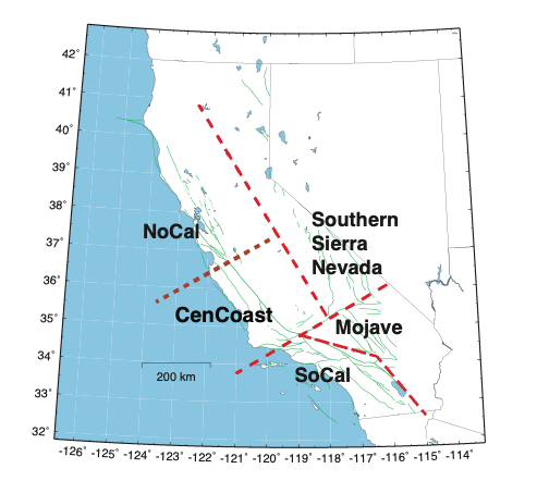
All five regions are installed in production. When an event's epicenter falls outside every native extent, the simulation runs against the geographically nearest installed region (an equirectangular distance to each region's extent) and the result is labeled an approximation — the map above shows which region that would be, even before it's picked. Location alone does not make an event ineligible: nothing in BBP validates that a rupture's tectonic style matches the crustal profile it runs against, so a Cascadia subduction-zone event, for example, is still simulated using a method built for shallow crustal ruptures, and that result is illustrative only. There are just two eligibility criteria: a magnitude of M5.0 or above, and at least one velocity-model region installed. Distance from a region's extent is not one of them — a Reno, Las Vegas, Portland or Mexicali earthquake is simulated against the nearest installed model and labeled an approximation, rather than being refused. Where an event falls below the magnitude floor, or a simulation fails or is unavailable, the animation falls back to the ShakeMap-driven empirical synthetic instead.

A separate 200 km limit does apply, but to a different distance: how far from the epicenter an individual site may be placed in the Simulation Lab, since that is the range over which the method is validated for a station. It constrains where you may ask for a seismogram; it has never governed whether the earthquake itself can be simulated.

Building the Site List

One BBP job per event covers every site its pending animations need: the closest qualifying gazetteer city (for the simulated animation) plus all three ground-motion-decay virtual sites, so every panel of the decay animation shares one stochastic rupture rather than confounding attenuation with rupture-to-rupture variability. Sites are supplied to BBP as a station list, each with site-specific V_s30 from the same UCVM-first lookup chain described in ShakeMap vs. GMPE Comparison — except the three decay panels, which are all simulated at V_S30 = 760 m/s (the NEHRP B/C rock reference) so that distance alone, not near-surface material, is what differs between them.

BBP returns three-component velocity and acceleration time series. Velocity is integrated once to displacement with baseline correction, then drives the shake scene through the same displacement pathway used for real recorded seismograms (see Physics Animation (Blender)). The three decay records are clipped to a single shared time window — earliest peak minus 5 s to latest peak plus 15 s — rather than each to its own peak, so the delay between panels is the simulation's own: the far site starts later and keeps shaking after the near site has settled because that is what the seismograms do, not because an arrival time was assumed.

Goodness-of-Fit: Scoring the Simulation Against Reality

A simulation that looks convincing in an animation is not necessarily accurate, so for each qualifying event Intensity Lab measures the simulation against the real earthquake. It retrieves the recorded accelerations at seismic stations around the epicenter (via the same ObsPy/FDSN pipeline described in Observed Seismic Station Data — though uncut acceleration for this comparison, not the clipped displacement used for animation), submits them alongside a BBP simulation of the same event, and reads back the Broadband Platform's own goodness-of-fit residuals — the mean logarithmic bias between the observed and simulated response spectra.

The result is published as a goodness-of-fit report, shown on the event page under BBP Simulation Comparison with a full report page of its own and a downloadable PDF, with a verdict against a pre-declared pass band (a factor of two, i.e. a mean absolute bias of 0.69). Because a structure responds at its own period, the report states the bias period by period rather than as a single average and flags any period outside the band — a simulation can pass on the mean while being well off at a specific period.

Standing Limitations

• These are visualizations, not hazard products. BBP seismograms shown in animations illustrate the character of shaking; they are not site-specific engineering ground motion estimates and should not be used for design.
• The rupture is derived, not observed. Fault dimensions come from magnitude scaling, and the moment tensor's conjugate nodal plane is equally consistent with the data — choosing it would produce different waveforms.
• Emulated hardware on Apple Silicon dev machines runs BBP under x86_64 emulation, so amplitudes there are not SCEC-reference-accurate; production runs natively.
• The nearest decay panel usually sits on the rupture. Decay animations sample 5, 50 and 100 km from the epicenter, and at the magnitudes that qualify the modelled fault is tens of kilometres long — so the 5 km site typically falls within the fault's surface projection, the near field where simulated amplitudes are most sensitive to the assumed rupture geometry and least constrained by the method's validation.

When BBP is unavailable, no velocity model is close enough, or the magnitude is below the floor, animations fall back automatically to the ShakeMap-driven synthetic. Animations rendered from a BBP seismogram are labeled as such in the video overlay.